Computers have always been notorious bad at text generation and comprehension. Anyone who’s ever had an unfortunate experience with autocorrect or “Google Translated” something into their native language will probably tell you that computers can’t write worth a damn. They can fix spelling and look up words in a dictionary, but they struggle to make sense of the sequential, contextual structure of language. So you can imagine my surprise when I sat down at my computer the other morning and found these lines written by a Recurrent Neural Network, or RNN, that I had thrown together the previous evening and left running overnight on my laptop CPU.

Okay, sure, it’s not really Shakespeare, but I’d forgive someone for mistaking it for an obscure quote from one of his later plays. And it wasn’t just that quote that struck me, but page after page of faux-Shakespeare from my hastily written network. Andrej Karpathy’s famous essay on the subject, The Unreasonable Effectiveness of Recurrent Neural Networks, is aptly named: RNNs are uncanny, strange, unpredictable, and sometimes beautiful. In this essay, I’d like to go through the basics of RNNs and LSTMs, provide some tips for implementing and training them, and talk about recent developments in the field. You can find the char-rnn responsible for this passage, and many more pages from this and other datasets in my Github LSTM repository.

What is an RNN?

RNNs, or Recurrent Neural Networks, are neural networks capable of sequential learning. For people new to machine learning, a neural network is simply a set of mathematical operations, usually linear matrix multiplications followed by non-linear activation layers, that resemble aspects of the human brain, and are trained on real-world data. Usually, they take a single input, like an image, and produce a single output, like a label (answering the question “what is this an image of?”, for example). RNNs are different - they take a sequence of inputs, and return an output or set of outputs that reflect the sequential, often temporal nature of the inputs.

While this may seem restrictive, something you quickly discover is that just about anything can be a sequence. It’s easy to see that words and sentences are sequential, but RNNs can also be used for everything from image generation to music composition to object classification. Humans are amazing at learning because we learn in context; we can remember and contextualize a word in a sentence that last appeared pages ago. We can even use knowledge acquired from one task to improve our performance on another, mostly unrelated one. Our neural networks should be able to do the same thing.

A typical RNN architecture will look something like this:

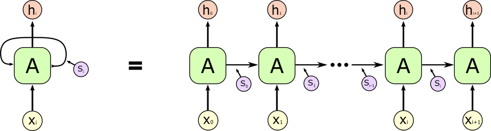
This may look complicated, but it’s actually pretty simple. The RNN is just a single cell (the green block labeled A) with an input (x), an output (h), and a state vector (s) which is updated every time a new input is processed. During training, a sequence of elements is fed one by one into the RNN, and the state vector is continually updated, acting as a sort of record of the past elements in the sequence. Since the weights inside the neuron “body” control both how it interprets and generates the state vector, it can learn via backpropogation how to more accurately and succinctly summarize and remember important information about previous inputs.

More technically, the basic RNN is a set of three weight matrices with associated bias vectors which are modified during training. Each input is encoded as a vector, either one-hot encoded or placed into an “embedding space” by a network that learns during training to assign more and more representative vectors to each input. The state and input vectors are supplied to linear layers (multiplied by a matrix $w$ and shifted by a bias $b$), and then, in the most common formulation, they are added to one another and normalized with a tanh activation.

This is as far as the state vector goes, but we need to add one more linear layer to decode the output, since generally the vectors will be longer than the input length while inside the RNN cell (we refer to the size of the input space as the input size and the size of the RNN state space as the RNN size or number of hidden nodes). This matrix $w_o$ will have shape (input_size, rnn_size).

Our loss function is just an $L^2$ or cross-entropy loss function measuring the distance between the output sequence and the desired results. The beautiful thing about RNNs is that the labels are actually just the input sequence shift right by one time-step, so the network learns to produce the next word in a sequence given prior elements. Backpropogation is not difficult, although the gradient associated with outputs later in the sequence will be quite long, since they depend on every input layer before them.

Implementation in Tensorflow

The LSTM cell is just a set of three matrices wi, ws, and wo with biases, applied to the inputs, state vector, and outputs, respectively. A Tensorflow pseudo-code implementation looks like this:

def RNN_cell(input, state):

  wi = tf.get_variable("wi", [input_size, rnn_size], initializer=...) # weight and bias for input
  bi = tf.get_variable("bi", [rnn_size], initializer=...)

  ws = tf.get_variable("ws", [rnn_size, rnn_size], initializer=...) # weight and bias for state vector
  bs = tf.get_variable("bs", [rnn_size], initializer=...)

  wo = tf.get_variable("wo", [rnn_size, vocab_size], initializer=...) # weight and bias for decoding RNN output
  bo = tf.get_variable("bo", [vocab_size], initializer=...)

  state = tf.nn.tanh(tf.nn.xw_plus_b(input, wi, bi) + tf.nn.xw_plus_b(state, ws, bs))
  output = tf.nn.xw_plus_b(state, wo, bo)

  return output, state

Easy-peasy. We create three sets of weight/bias variables, wi/bi, ws/bs, and wo/bo, use two of them to rescale and shift the input and state vector, and then apply the tanh normalization and generate the output using a third layer. RNNs can also be stacked on top of each other, so the output sequence is used as the input sequence for another RNN. To do this, we just call the RNN_cell recursively: output, state = RNN_cell(RNN_cell(input, state)). Since I had a hard time implementing this, I’ll add a diagram of the two layer RNN model:

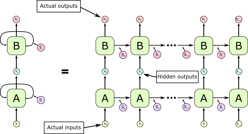
This adds an arbitrary amount of depth to the model, and makes the RNN rather more reminiscent of human memory, where memory is handled by many different neurons with different functions. We can also add activations or even entire new layers between the layers of the RNN. Since we usually want our network to predict subsequent elements in our input sequence, we train our network to produce outputs equal to the next input, i.e. to make $h_0$ equal to $x_1$, $h_1$ equal to $x_2$, etc. That elegance is what makes RNNs so powerful and easy to use - we don’t need any training data beyond the actual text of the dataset. In Tensorflow, the labels and input data looks like this:

train_data = list() # here we take a sequence of characters from the training data and store them in a list
for _ in range(sequence_length + 1):
  train_data.append(tf.placeholder(tf.float32, shape=[batch_size, vocabulary_size]))
inputs = train_data[:sequence_length]
train_labels = train_data[1:]

If our training data is a long block of text, we select sequences of length sequence_length at random from the text to limit the length of the backpropogation graph. If we tried backpropogating over the entire corpus, the graph would grow exponentially, and gradients for distant inputs would quickly vanish. Next we create an initial state variable, and repeatedly apply the RNN_cell to our inputs, modifying the state variable each time. At the end, we convert our output list into a tensor, and apply a standard loss function.

state = tf.constant(shape=[rnn_size]) # initial state vector

outputs = [] # list for storing outputs

for element in inputs:
  with tf.variable_scope("RNN") as scope:
    state, output = RNN_cell(element, state)
    scope.reuse_variables()
    outputs.append(output)

logits = tf.pack(outputs) # convert list into tensor

loss = tf.reduce_mean(tf.nn.softmax_cross_entropy_with_logits(
                            labels=tf.concat(train_labels, 0), logits=logits)

predictions = tf.nn.softmax(logits)

The model is then trained on a standard SGD optimizer (classical SGD, or Adam/RMSProp/others).

LSTMs: What’s the Big Deal?

We have a working model right now, but it has some major drawbacks. For one thing, it’s very shallow, and these normalized linear layers aren’t capable of capturing much complexity in the state space. For another things, the addition of a single state vector is a very crude way of handling memory, since information about older elements is lost as the network optimizes for relatively more important shorter-term memory. These problems are rectified by the LSTM (Long Short-Term Memory) model.

An LSTM is an RNN unit with a clever mechanism for learning what to remember and what to forget. To do this, we add aptly-named forget and memory gates, which control how the state vector is interpreted and modified inside the LSTM.

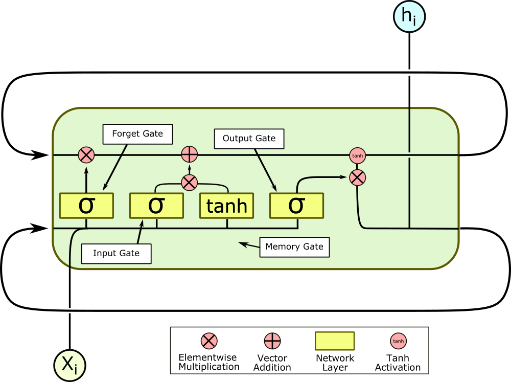
The yellow squares, in order from left to right, are the forget, input, memory, and output gates, and they each have a specific function. The first gate is the forget gate, which controls what information in the state vector is allowed back into the LSTM cell. The previous output $o_{i-1}$ is fed back into the cell, concatenated with the new input $x_i$, and fed through a linear layer with a sigmoid activation.

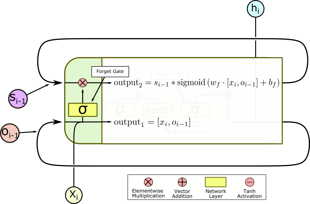
The sigmoid activation normalizes the output of the layer to between zero and one, so when the new vector is multiplied elementwise by the state vector, each element is re-prioritized; parts of the vector can be left virtually untouched, while others are totally erased. This gate allows the cell to forget features of the previous inputs which it doesn’t care very much about, and keep features it thinks are important, by rescaling the corresponding element of the state vector.

The second gate is the input gate, and it is also a sigmoid layer, but unlike the forget gate, it controls how much the state vector is actually updated by the new input and previous outputs. Instead of multiplying the state vector, it multiplies the output of the next gate, the memory gate, which rescales and normalizes the concatenated input and output vector, before they are added elementwise to the state vector.

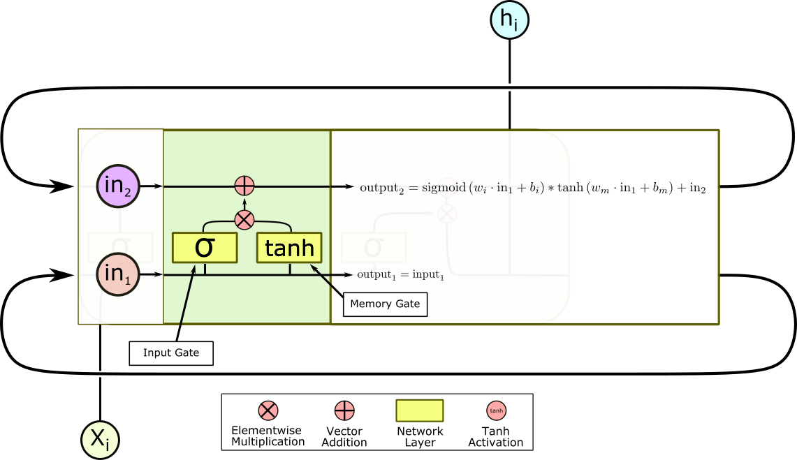
This pair of gates controls long-term learning. If a particular input is an outlier, these two gates can effectively ignore it. And even if an input isn’t relevant right now, it can pass through these gates and modify the state vector, without changing this output. These gates are what makes LSTMs great at making long-term associations. From here, the state vector is sent out of the cell and reenters to repeat the process all over again. However, we aren’t quite done yet.

In the last step, the concatenated input and prior output are transformed by the final output layer, normalized by a sigmoid activation, and multiplied elementwise by the state vector, which itself has been normalized by a tanh activation.

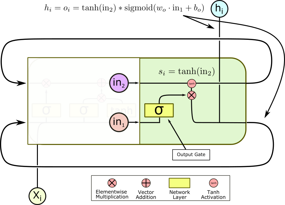
This final gate again allows the cell to ignore aspects of the previous sequence which may be relevant for future entries, but aren’t relevant to this output. At last, we are done, and one final linear layer outside the cell can decode the output and get us our actual result, whether it’s a word, a letter, or an array of pixels.

LSTM implementation in Tensorflow

The LSTM body method looks very similar to the simple RNN, with the addition of two new layers. I’ve removed the decoding output layer that I included in the RNN method for the sake of reusability.

def lstm_cell(i, o, state):
    # Input gate: input, previous output, and bias.
    x = tf.get_variable("x", [vocabulary_size, 4 * num_nodes],
                         initializer=tf.truncated_normal_initializer(-0.1, 0.1, dtype=tf.float32))
    m = tf.get_variable("m", [num_nodes, 4 * num_nodes],
                         initializer=tf.truncated_normal_initializer(-0.1, 0.1, dtype=tf.float32))

    ib = tf.get_variable("ib", [1, num_nodes], initializer=tf.zeros_initializer(dtype=tf.float32))
    fb = tf.get_variable("fb", [1, num_nodes], initializer=tf.zeros_initializer(dtype=tf.float32))
    cb = tf.get_variable("cb", [1, num_nodes], initializer=tf.zeros_initializer(dtype=tf.float32))
    ob = tf.get_variable("ob", [1, num_nodes], initializer=tf.zeros_initializer(dtype=tf.float32))

    xtemp = tf.matmul(i, x)
    mtemp = tf.matmul(o, m)

    ix, fx, cx, ox = tf.split(xtemp, 4, axis=1)
    im, fm, cm, om = tf.split(mtemp, 4, axis=1)

    input_gate = tf.sigmoid(ix + im + ib)
    forget_gate = tf.sigmoid(fx + fm + fb)
    update = cx + cm + cb
    state = forget_gate * state + input_gate * tf.tanh(update)
    output_gate = tf.sigmoid(ox + om + ob)

    return output_gate * tf.tanh(state), state

We use matrices x and m of size vocabulary_size x 4 * num_nodes to avoid 4 separate matrix multiplications. Instead, we can just multiply the input once by a matrix four times as large, and then split the output for use in the appropriate gates. When it actually comes to implementing a multilayer LSTM, the implementation gets a little hairier, because the state vector needs to be saved between layers. First of all, for each layer, we need weight and bias variables to serve as an intermediate layers. I choose to save some effort and make these weights have an output dim equal to the vocabulary size, but this is not necessary. We repeatedly call the lstm_cell, but we need to explicitly allow reused variables, so Tensorflow knows that we really want to “get” the same variable. After each loop, we assign the outputs of each layer to saved_output and saved_state` variables, which are used as the initial output and state variables the next time the loop is run.

for j in range(num_layers):
    with tf.variable_scope('layer{}'.format(j)) as scope:
        w = tf.get_variable("w", [num_nodes, vocabulary_size],
                            initializer=tf.truncated_normal_initializer(-0.1, 0.1, dtype=tf.float32))
        b = tf.get_variable("b", [vocabulary_size], initializer=tf.zeros_initializer(dtype=tf.float32))

        saved_output = tf.get_variable("saved_output", [batch_size, num_nodes],
                                       initializer=tf.zeros_initializer(dtype=tf.float32), trainable=False)
        saved_state = tf.get_variable("saved_state", [batch_size, num_nodes],
                                      initializer=tf.zeros_initializer(dtype=tf.float32), trainable=False)

        outputs = list()
        output = saved_output
        state = saved_state

        for i in inputs:
            output, state = lstm_cell(i, output, state)
            scope.reuse_variables()
            outputs.append(output)

        # State saving across unrollings.
        with tf.control_dependencies([saved_output.assign(output), saved_state.assign(state)]):
            # Classifier.
            logits = tf.nn.xw_plus_b(tf.concat(outputs, 0), w, b)

            if j != num_layers - 1:
                _logits = tf.reshape(logits, [num_unrollings, batch_size, vocabulary_size])
                inputs = tf.unstack(tf.nn.softmax(_logits))

            if j == num_layers - 1:
                loss = tf.reduce_mean(
                    tf.nn.softmax_cross_entropy_with_logits(
                        labels=tf.concat(train_labels, 0), logits=logits))

In order to compute the loss, we multiply the last output of the uppermost layer by a weight and bias, and then apply a cross entropy loss function. We perform some clever concatenation and reshaping here to handle training in batches.

Training LSTMs

LSTMs are sometimes thought to be difficult to train, but in truth that tends not to be the case. They can be slow to train, but they don’t have the unfortunate tendency of diverging wildly when the learning rate is even a little too high, like many CNNs and GANs. The key in my experience to rapid, efficient training is a shallow network (2 layers, 128 hidden layers, .002 learning rate on Adam or RMSProp). This will achieve very respectable results very rapidly, but will saturate at a certain point (around 30000 iterations in my experience). Better results come with a serious performance cost: going up to 3 layers immediately slows training by several orders of magnitude, and increasing the number of hidden units to 512 or 1024 increases the number of parameters by a factor of 16 and 32 respectively, compared to the 128 units network. However, achieving anything more than a superficial resemblance to a dataset requires a large number of hidden units and multiple layers, so it’s often worth the time.

Recent developments

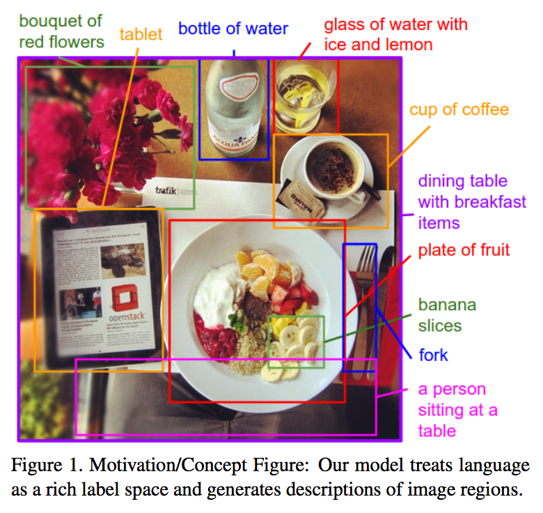
LSTMs have been around for a while, but they’re still an extremely active field of research. Several variants of the LSTM have been popularized over the years, including LSTMs with peepholes, which are learned connections between the various gates, and GRUs, developed by Cho, et al. (2014), which scrap the independent forget gate and use the input gate for both purposes instead. This makes them much faster to train, and seems to have very little adverse effect on network efficacy. LSTMs are also being used more and more in other machine learning tasks, like image recognition, labeling, and generation. Li Fei-Fei and Andrej Karpathy used LSTMs. to caption images in context, localizing objects with a convolution network, and then inserting those region classifications into an LSTM which produced contextual labels.

The 2015 Gregor et al. paper DRAW: A Recurrent Neural Network For Image Generation used RNNs to generate images, like handwritten letters from MNIST, sequentially, focusing the generative network’s attention on a single small region of the image at a time, much like humans do when drawing numbers or pictures.

Visualization

Like in convolution networks, the ability of such neural networks to summarize and perform “unsupervised learning” is quite extraordinary, and visualizing the activations of a fully trained LSTM can be linguistically fascinating. These visualizations can be performed using Tensorflow’s Tensorboard suite, and can identify “trigger words” or phrases, sequences of characters which strongly encourage the network to produce a certain output. These can be common phrases, interjections, or even words which fit within the meter of the passage. Karpathy’s essay is an excellent resource for more information on this subject.

All in all, LSTMs are an exciting, powerful, and sometimes beautiful tool for sequential learning that can be easily and conveniently implemented in Tensorflow or Keras. I hope this was helpful, and feel free to ask any questions in the comments.

I’d like to thank a number of friends for giving me feedback on this post, and Andrej Karpathy and Christopher Olah for inspiring the essay and many of the graphics used to illustrate concepts!